2nd Order Dynamic Systems

Response of Second Order Systems

For a similar mass damper system to what was presented in 1st Order Dynamic Systems…

Nomenclature

Sometimes dampers are b, sometimes they are c…

Starting with out 2nd order ODE…

• $m{x}^{{}^{\prime \prime }}+c{x}^{\prime }+kx=f\left(x\right)$
• Taking a LaPlace transform
• $m[s^{2}X\left(s\right)-sx\left(0\right)-x^{\prime }\left(0\right)]+c\left[sx\left(s\right)-x\left(0\right)\right]+kX\left(s\right)=F\left(s\right)$
• Factoring out X(s) and F(s) we can derive the following to get to the transfer function
• $X\left(s\right)=\frac{F\left(s\right)}{m{s}^2+cs+k}+\frac{msx\left(0\right)+m{x}^{\prime }\left(0\right)+cx\left(0\right)}{m{s}^2+cs+k}$
  • $\frac{X\left(s\right)}{F\left(s\right)}=\frac{1}{m{s}^2+cs+k}$

*You can use the auxiliary method from State Variable Models if you have a time differentiated input

Standard Form

Step response: $G\left(s\right)=k\frac{{\omega }_n^2}{s^2+2\zeta {\omega }_{n}s+{\omega }_n^2}$

• Where the denominator can be factored as… ${\left(s+\sigma \right)}^2+{\omega }_d^2$

There are different cases here which are the Free Damped Responses.

• Final value (DC gain): k
• Peak time $T_p=\frac{\pi }{{\omega }_n\sqrt{1-{\zeta }^2}}$
• Settling time (5%)
  • $T_s=\frac{3.2}{\zeta {\omega }_n},0<\zeta <0.69$ OR $T_s=\frac{4.5\zeta }{{\omega }_n},\zeta >0,69$
  • $e_{}^{-\zeta {\omega }_n{t}_s}=0.05$
  • $t_s=\frac{4}{|\sigma |}$ (2% settling time which is for 1st Order Dynamic Systems!!!! need to relocate this) Rise time:
• $T_r=\frac{0.8+2.5\zeta }{{\omega }_n}$
• $t_r\cong \frac{1.8}{{\omega }_n}$ Side note: $\theta ={\cos }^{-1}\left(\zeta \right)$ and $\sigma =\zeta {\omega }_n$ and ${\omega }_d={\omega }_n\sqrt{1-{\zeta }^2}$

Finding poles on a graph

Find ${\omega }_n$ which is the unit circle distance, then find $\zeta$ which is the angle (direction) of the poles, then find $\sigma$ which is the vertical distance away from the imaginary axis to which the poles lie.

For an undamped 2nd order response
When c=0…
$X\left(s\right)=\frac{F\left(s\right)}{m{s}^2+k}+\frac{m{x}^{\prime }\left(0\right)+msx\left(0\right)}{m{s}^2+k}$
$X\left(s\right)=\frac{\frac{F\left(s\right)}{m}}{s^2+\frac{k}{m}}+\frac{x^{\prime }\left(0\right)+sx\left(0\right)}{s^2+\frac{k}{m}}$
Where the terms above are out zero state response and zero input response

Zero Input Response

• $X_{zir}\left(s\right)=\frac{x^{\prime }\left(0\right)}{s^2+\frac{k}{m}}+\frac{sx\left(0\right)}{s^2+\frac{k}{m}}\frac{}{}$

Transfer Function

• $\frac{X\left(s\right)}{F\left(s\right)}=\frac{\frac{1}{m}}{s^2+\frac{k}{m}}$

Where the “characteristic equation” models our poles.

Using the characteristic equation, we can derive the natural frequency of the system as…

• ${\omega }_n=\sqrt{\frac{k}{m}}$
• $X\left(s\right)=\frac{x^{\prime }\left(0\right)}{s^2+{\omega }_n^2}+{\frac{sx\left(0\right)}{s^2+{\omega }_n^2}}_{}$
• $X\left(s\right)=\frac{x^{\prime }\left(0\right)}{{\omega }_n}{\frac{{\omega }_n}{s^2+{\omega }_n^2}}_{}+x\left(0\right)\frac{s}{s^2+{\omega }_n^2}$

Using this inverse LaPlace transform from LaPlace Transforms…

• $\cos \left(bt\right)u\left(t\right)=\frac{s}{s^2+b^2}$
• $\sin \left(bt\right)u\left(t\right)=\frac{b}{s^2+b^2}$

Therefore, applying this concept…

• $x\left(t\right)=\left[\frac{x^{\prime }\left(0\right)}{{\omega }_n}\right]\sin \left({\omega }_{n}t\right)+x\left(0\right)\cos \left({\omega }_{n}t\right)]u\left(t\right)$
• Where this oscillates with the frequency of the poles

Also note the general solution for a 2nd order homogenous equation with $r=\pm \omega j$
$x\left(t\right)=B\sin \left(\omega t+\varphi \right)$
Using given boundary conditions, we can find $B$ and $\varphi$ by seeing which values satisfy the B.Cs

% Overshoot

This is the amount that the waveform overshoots the steady-state value…

• $\%OS=\frac{y_{\max }-y_{final}}{y_{final}}\cdot 100=e^{-\frac{\zeta \pi }{\sqrt{1-{\zeta }^2}}}\ast 100=M_p\ast 100$
• $y_{\max }=k\left(1+e^{-\frac{f\pi }{\sqrt{1-{\zeta }^2}}}\right)$
• $\zeta =\frac{-\ln \left(M_p\right)}{\sqrt{{\pi }^2}+{\ln }^2\left(M_p\right)}$
• We also use these identities
  • $\tan \theta =\frac{\zeta }{\sqrt{1-{\zeta }^2}}$
  • $\zeta =\sin \theta$

Damped Response

The Characteristic equation is defined as
$m{s}^2+cs+k=0$
$s^2+\frac{c}{m}s+\frac{k}{m}=0$

Damped Response Important Variables

Where we have these relationships…

• $\frac{c}{m}=2\zeta {\omega }_n$ or $\zeta =\frac{c}{2m{\omega }_n}\frac{c}{c_{cr}}$
• $c_{cr}=2m{\omega }_n=2\sqrt{km}$ which means $\zeta =\frac{c}{2\sqrt{km}}$ and
• $s=-\zeta {\omega }_n\pm {\omega }_n\sqrt{{\zeta }^2-1}$ are the poles
• Note that $s=-\zeta {\omega }_n\pm j{\omega }_d$ as well where ${\omega }_d={\omega }_n\sqrt{1-{\zeta }^2}$ or the imaginary part of the poles

The Free Damped Response

$X\left(s\right)=\frac{sx\left(0\right)+x^{\prime }\left(0\right)+\frac{c}{m}x\left(0_{}\right)}{s^2+2\zeta {\omega }_n+{\omega }_{n^2}}$
Where the poles are given above.

Case 1

If $\zeta >1$, then $c>2\sqrt{km}$ and $\sqrt{{\zeta }^2-1}>0$ which is the over-damped case.

and our discriminate is positive meaning we have two distinct real poles.
This yields…
$X\left(s\right)=\frac{sx\left(0\right)+x^{\prime }\left(0\right)+2\zeta {\omega }_{n}x\left(0\right)}{\left(s-s_1\right)\left(s-s_2\right)}$
$x\left(t\right)=C_1{e}^{s_{1}t}+c_2{e}^{s_{2}t}$
Where $\{\begin{array}{l}{\tau }_1=\frac{-1}{s_1}\\ {\tau }_2=\frac{-1}{s_2}\end{array}$
and ${\tau }_2>{\tau }_1$ meaning that $s_2$ is the dominant pole.

Solving

After coupling the system, solve for the s’s and the time constant above, then…
${\omega }_n=\sqrt{s_1{s}_2}$
$\zeta =\frac{s_1+s_2}{2{\omega }_n}$

Case 2

$\zeta =1$ then $c=c_{cr}$, this represents the critically damped case. This is the minimum damping to have no oscillation.

${\zeta }^2-1=0$ in this case and $s=-\zeta {\omega }_n\pm 0$ yields repeated real poles.

in this case, $s=-{\omega }_n$
Using the derivation from the lectures…
$x\left(t\right)=\left(c_1+c_2\right)e^{st}=\left(c_1+c_2\right)e_{}^{-{\omega }_{n}t}$

Note

No ${\omega }_n$ or ${\omega }_d$ since there is no oscillation

Case 3

$0<\zeta <1$ represents the underdamped case. This should yield imaginary roots.
$c<2\sqrt{\mathrm{km}}$

$s=-\zeta {\omega }_n\pm j{\omega }_n\sqrt{1-{\zeta }^2}$ where ${\omega }_d$ is the natural frequency and the square root term.

$e_{}^{-\zeta {\omega }_{n}t}\left[\cos {\omega }_{d}t+=\zeta \sin {\omega }_{d}t\right]$

From the line above $\tau =\frac{1}{\zeta {\omega }_n}=\frac{2m}{c}$

$x\left(t\right)=C_1{e}^{s_{1}t}+C_2{e}^{s_{2}t}$
$x\left(t\right)=e^{-\zeta {\omega }_{n}t}\left[A\sin \left({\omega }_{d}t\right)+x\left(0\right)\cos \left({\omega }_{d}t\right)\right]$ where $A=\frac{\zeta }{\sqrt{1-{\zeta }^2}}x\left(0\right)+\frac{1}{{\omega }_d}{x}^{\prime }\left(0\right)$

Where $s_1^{\ast }=s_2$ with maybe some error

Solving

Useful equations for this case…
${\omega }_n=\sqrt{Re{\left(s\right)}^2+Im{\left(s\right)}^2}$
${\omega }_d={\omega }_n\sqrt{1-{\zeta }^2}$ $\zeta =\frac{-Re\left(s\right)}{{\omega }_n}$ $\tau =-\frac{1}{\mathrm{Re}\left(s\right)}$
$\sin \theta -\sqrt{1-{\zeta }^2}=\sqrt{1-\cos {\theta }^2}$
$G\left(s\right)=k\frac{{\omega }_n^2}{s^2+2\zeta {\omega }_{n}s+{\omega }_n^2}$

---

Effects of Pole Locations

For qualitative understandings, will not be examinable though…

• As you move further away from the imaginary axis, overshoot decreases and our damping increases
• Increasing ${\omega }_d$ increases frequency but keeps the same overshoot
• As $\zeta$ decreases, ${\omega }_d$ increases which increases frequency but yields a similar envelope as we make these changes Adding poles:
• Poles dominate if they are close to zero (often converts a 2nd order system to a 1st order system)
• If close to real parts of other poles, the response slows down

Effects of Zeroes

Also for qualitative effects
Adding zeroes:

• Adding zeroes in the numerator increases the overshoot the closer the zero is to the real axis
  • If its far away from the axis, basically nothing happens
• If we have a zero in the same location as a pole, they effectively cancel each other out

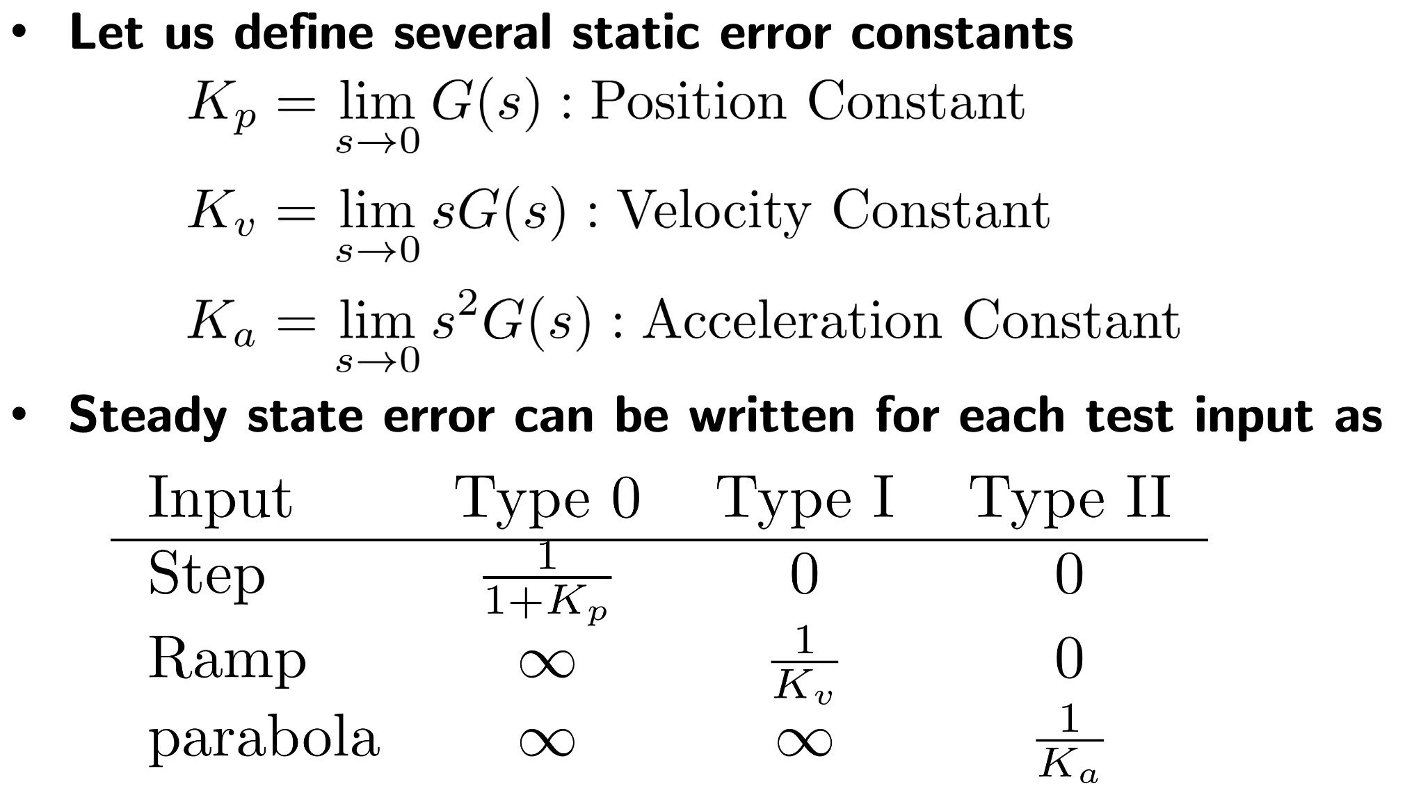
System Types

The type of a system is the number of poles it has at the origin…

• Type 0 → No poles
• Type 1 → 1 pole
• Type 2→ 2 poles

Increasing System Type

The simplest way to increase the system type is to add an s to the denominator of the open-loop TF. or to add a $\frac{1}{s}$ block to the block diagram